Rendering blank image

Let’s start to use Lightmetrica by rendering a blank image. We first import the lightmetrica module, where we use lm as an alias of lightmetrica for simplicity.

Note

Although we recommend to use Python API to organize the experiments, similar APIs can be accessible from C++. See example directory for the detail.

Note

lmenv is a simple module to configure Lightmetrica envrionment from a specified file. Here we load .lmenv. You want to create your own .lmenv file if you want to execute examples or tests by yourself. For detail, please refer to Executing functional tests.

import lmenv
lmenv.load('.lmenv')

Namespace(bin_path='/lightmetrica-v3/_build/bin', path='/lightmetrica-v3', scene_path='/lm3/scenes')

import lightmetrica as lm

Lightmetrica offers an extension for the Jupyter notebook to support logging or interactive progress reporting inside the notebook. The extension can be loaded by a line magic command as below.

%load_ext lightmetrica_jupyter

After importing the module, you can initialize the framwork by calling lm::init() function. You can pass various arguments to configure the framework to the function, but here we keep it empty so that everything is configured to be default.

lm.init()

Logging and progress reporting in Jupyter notebook can be enabled by lm::log::init() and lm::progress::init() functions with corresponding types.

lm.log.init('jupyter')
lm.progress.init('jupyter')

Once the framework has been initialized properly, you can get an splash message using lm::info() function.

lm.info()

[I|0.005] Lightmetrica -- Version 3.0.0 (rev. 70601db) Linux x64

Next we define assets necessary to execute renderer, like materials, meshes, etc. In this example, we only need a film to which the renderer outputs the image. We can define assets by lm::load_* function, where * represents the name of the asset. In this example, we want to make film asset. So we use lm::load_film() function.

The first argument (film) specifies id of the asset to be referenced. The second argument (bitmap) is given as the type of the assets. The optional keyword arguments specify the parameters passed to the instance.

For convenicence, we will refer to the asset of the specific type in <asset type>::<name> format. For instance, film::bitmap represents a bitmap film asset. film::bitmap takes two parameters w and h which respectively specify width and height of the film.

This function returns a reference to the asset. You can access the underlying member functions. You can find details in API reference.

film = lm.load_film('film', 'bitmap', w=1920, h=1080)

[I|0.013] Loading asset [name='film']

The created instance of the asset is internally managed by the framework. Lightmetrica uses component locator to access the instance.

A component locator is a string starting with the character $ and the words connected by .. A locator indicates a location of the instance managed by the framework. For instance, the locator of the film asset is $.assets.film. This can be queried by .loc() function.

film.loc()

'$.assets.film'

To rendering an image, we need to create renderer asset. Here, we will create renderer::blank renderer. renderer::blank is a toy renderer that only produces a blank image to the film. The renderer takes film parameter to specify the film to output the image, and color parameter for the background color.

A reference to the other asset as a parameter can be passed using component locator. Here we use film.loc() to get a locator of the film. Althernaively, you can directly pass the instance of the asset directly as a parameter.

renderer = lm.load_renderer('renderer', 'blank',
    output=film,  # or alternatively, film.loc()
    color=[1,1,1]
)

[I|0.106] Loading asset [name='renderer']

lm::Renderer::render() function executes rendering.

renderer.render()

After rendering, the generated image is kept in film. lm::Film::save() function outputs this film to the disk as an image.

film.save('blank.png')

[I|0.376] Saving image [file='blank.png']

True

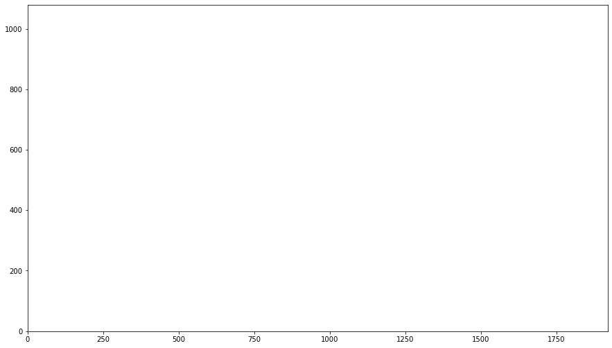
You can also visualize the film directly in Jupyter notebook. lm::Film::buffer() gets the internal image data as numpy array which you can visualize using matplotlib. We rendered a white blank image thus the following image is as we expected.

import numpy as np
%matplotlib inline
import matplotlib.pyplot as plt

img = np.copy(film.buffer())
f = plt.figure(figsize=(15,15))
ax = f.add_subplot(111)
ax.imshow(np.clip(np.power(img,1/2.2),0,1), origin='lower')
plt.show()

Finally, we gracefully shutdown the framework with lm::shutdown() function. Usually you don’t want to explicitly call shutdown function.

lm.shutdown()